Calculus
Introduction
Calculus is one of the most powerful and fundamental branches of mathematics, dealing with change and motion. At its core, calculus is the study of how things change, enabling us to understand the rates at which quantities increase or decrease and to calculate the total accumulation of quantities. It is divided into two main areas: differential calculus and integral calculus. Differential calculus focuses on rates of change, such as the slope of a curve or the velocity of an object, while integral calculus deals with accumulation, like finding the area under a curve or the total distance traveled.
A Brief History: The Calculus Controversy
The development of calculus is attributed to two of the greatest mathematicians in history: Sir Isaac Newton and Gottfried Wilhelm Leibniz. Both independently developed the fundamental principles of calculus in the late 17th century, though their approaches and notations differed significantly. Newton, working primarily in England, developed calculus to solve problems related to motion and gravitation. He called his method “the method of fluxions,” focusing on the concept of instantaneous rates of change.
Meanwhile, Leibniz, working in continental Europe, developed a more formalized system with a different notation, which is the one we predominantly use today. His work on the infinitesimal calculus provided a more rigorous foundation for the subject, focusing on the sum of infinitely small quantities.
This simultaneous development led to a bitter dispute over the invention of calculus, often referred to as the “Calculus Controversy” or the “War of Calculus.” Newton’s followers accused Leibniz of plagiarism, while Leibniz’s supporters claimed the opposite. Despite the controversy, both Newton and Leibniz’s contributions were monumental, and modern calculus is a synthesis of their ideas.
Today, calculus is essential in a wide range of fields, from physics and engineering to economics and biology. It provides the mathematical tools needed to model and analyze systems that change continuously, making it a cornerstone of modern science and technology.
In this course, we will embark on a journey through the fundamental concepts of calculus like to limits, derivatives, and integrals. By the end, we’ll have a solid understanding of how calculus can be used to solve real-world problems and model continuous change. Let’s dive in!
Functions and models
The fundamental objects that we deal with in calculus are functions.
A function $f$ is a rule that assigns to each element $x$ in a set $D$ exactly one element, called $f(x)$, in a set $E$.
We usually consider functions for which the sets $D$ and $E$ are sets of real numbers. The set $D$ is called the domain of the function. The number $f(x)$ is the value of $f$ at $x$ and is read “$f$ of $x$.” The range of $f$ is the set of all possible values of $f(x)$ as $x$ varies throughout the domain. A symbol that represents an arbitrary number in the domain of a function is called an independent variable. A symbol that represents a number in the range of $f$ is called a dependent variable. In Example A, for instance, $r$ is the independent variable and $A$ is the dependent variable.
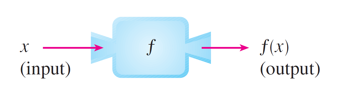
Figure 2: Machine diagram for a function $ƒ$
It’s helpful to think of a function as a machine (see Figure 2). If $x$ is in the domain of the function $f$, then when $x$ enters the machine, it’s accepted as an input and the machine produces an output $f(x)$ according to the rule of the function. Thus we can think of the domain as the set of all possible inputs and the range as the set of all possible outputs.
![]()
Figure 3: Arrow diagram for $ƒ$
Another way to picture a function is by an arrow diagram as in Figure 3. Each arrow connects an element of $D$ to an element of $E$. The arrow indicates that $f(a) = b$, $f(c) = d$, $f(e) = a$, and so on.
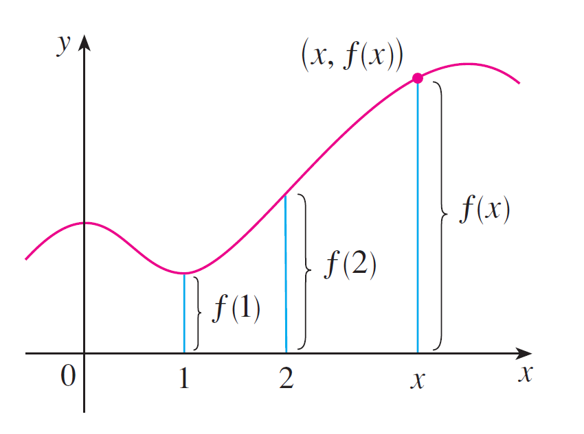
The most common method for visualizing a function is its graph. If $f$ is a function with domain $D$, then its graph is the set of ordered pairs \(\{(x, f(x)) \mid x \in D \}.\) (Notice that these are input-output pairs.) In other words, the graph of $f$ consists of all points $(x, y)$ in the coordinate plane such that $y = f(x)$ and $x$ is in the domain of $f$.
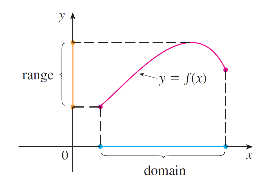
The graph of a function gives us a useful picture of the behavior or “life history” of a function. Since the $y$-coordinate of any point on the graph is $f(x)$, we can read the value of $f(x)$ from the graph as being the height of the graph above the point $x$ (see Figure 4). The graph of $f$ also allows us to picture the domain of $f$ on the $x$-axis and its range on the $y$-axis as in Figure 5.
 |  |
| Figure 4 | Figure 5 |
Representation of functions
There are four possible ways to represent a function:
- Verbally (by a description in words)
- Numerically (by a table of values)
- Visually (by a graph)
- Algebraically (by an explicit formula)
If a single function can be represented in all four ways, it’s often useful to go from one representation to another to gain additional insight into the function. But certain functions are described more naturally by one method than by another.
The graph of a function is a curve in the $xy$-plane. But the question arises: Which curves in the -plane are graphs of functions? This is answered by the following test.
The vertical line test: A curve in the $xy$-plane is the graph of a function of $f$ if and only if no vertical line intersects the curve more than once.